
 About Authors:
Ram Chandra*, Abhimanyu, Dr. Ashutosh Aggarwal
Seth G.L. Bihani S.D. College of Technical Education,
Institute of Pharmaceutical Sciences and Drug Research,
Sri Ganganagar, Rajasthan, INDIA
*rcgedar@gmail.com
1. Introduction
Biostatistics is contraction of biology and statistics, sometimes referred to as biometry or biometrics, is the application of statistics to a wide range of topics in biology. The science of biostatistics encompasses the design of biological experiments, especially in medicine and agriculture; the collection, summarization, and analysis of data from those experiments; and the interpretation of, and inference from, the results. Hypothesis testing determines the validity of the assumption with a view to choose between two conflicting hypotheses about the value of a population parameter. Hypothesis testing helps to decide on the basis of a sample data, whether a hypothesis about the population is likely to be true or false. Statisticians have developed several tests of hypotheses (also known as the tests of significance) for the purpose of testing of hypotheses which can be classified as:- (a) Parametric tests or standard tests of hypotheses, and (b) Non-parametric tests or distribution-free test of hypotheses. Parametric tests usually assume certain properties of the parent population from which we draw samples. Assumptions like observations come from a normal population, sample size is large, assumptions about the population parameters like mean, variance, etc., must hold good before parametric tests can be used. But there are situations when the researcher cannot or does not want to make such assumptions. In such situations we use statistical methods for testing hypotheses which are called non-parametric tests because such tests do not depend on any assumption about the parameters of the parent population. Besides, most non-parametric tests assume only nominal or ordinal data, whereas parametric tests require measurement equivalent to at least an interval scale. (Bolton Sanford 2004, Jakel James et.al. 2001)
[adsense:336x280:8701650588]
Reference Id: PHARMATUTOR-ART-1546
2. Student t- test
Student t-test is based on t-distribution and is considered an appropriate test for judging the significance of a sample mean or for judging the significance of difference between the means of two samples in case of small sample(s) when population variance is not known (in which case we use variance of the sample as an estimate of the population variance). In case two samples are related, we usepaired t-test (or what is known as difference test) for judging the significance of the mean of difference between the two related samples. It can also be used for judging the significance of the coefficients of simple and partial correlations. The relevant test statistic, t, is calculated from the sample data and then compared with its probable value based ont-distribution (to be read from the table that gives probable values of t for different levels of significance for different degrees of freedom) at a specified level of significance for concerning degrees of freedom for accepting or rejecting the null hypothesis. It may be noted that t -test applies only in case of small sample(s) when population variance is unknown.
2.1 Use of t-test
In medical research, t-test is among the three or four most commonly use statistical tests. The purpose of a t-test is to compare the means of a continuous variable in two research samples in orders to determine whether or not the difference between the two observed means exceeds the difference that would be expected by chance from random samples. (Jakel James et.al 2001, Kothari C.R. 1990).
2.2 Some important terms used in student t –test
(i) Degree of freedom-
The term degree of freedom refers to the number of observations that are free to vary. The degrees of freedom for any tests are considered to be the total sample size minus 1 degree of freedom for each mean that is calculated. In the student’s t-test, 2 degree of freedom are lost because two means are calculated one mean for each group whose means are to be composed. The general formula for the degrees of freedom for the student’s two group t-test is N1 + N2 – 2, where N1 is the sample size in the first group and N2 is the sample size in the second group. (Jakel James et.al. 2001, Armstrong N et.al. 2006)
(ii) The t-distribution
The t-distribution was described by William Goasset, who used the pseudonym “student” when he wrote the description. The normal distribution is the z distribution. The t distribution looks similar to it, except that its tails are somewhat wider and its peak is slightly less high, depending on the sample size. The t-distribution is necessary because when sample size. The t distribution is necessary because when sample sizes are small, the observed estimates of mean and variance are subject to considerable error. The larger the sample size is the smaller the errors are and the more the t size distribution looks like the normal distribution. In the case of an infinite sample size, the two distributions are identical. For practical purposes, when the combined sample size of the two groups being compared is larger than 120, the difference between the normal distribution and the t distribution is negligible. (Jakel James et.al. 2001, Le Chap T 1992)
2.3 Technique to perform test
1. Weneed to construct a null hypothesis - an expectation - which the experiment was designed to test. For example:- If we are analysing the heights of pine trees growing in two different locations, a suitable null hypothesis would be that there is no difference in height between the two locations. The student's t-test will tell us if the data are consistent with this or depart significantly from this expectation. So it is sensible to have a null hypothesis of "no difference" and then to see if the data depart from this.
2. List the data for sample (or treatment) 1.
3. List the data for sample (or treatment) 2.
4.Record the number (n) of replicates for each sample (the number of replicates for sample 1 being termed n1 and the number for sample 2 being termed n2)
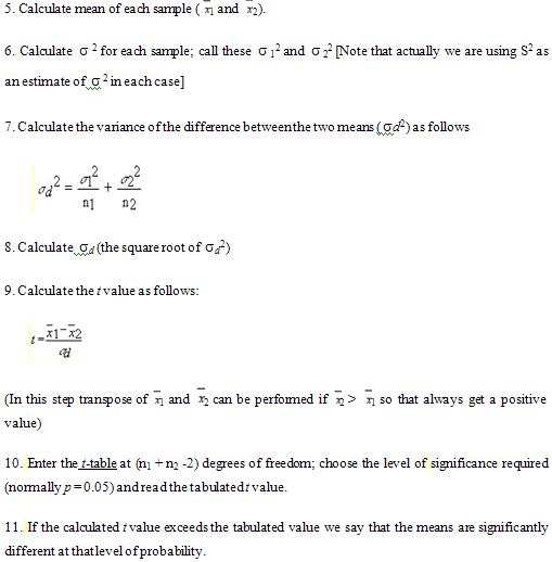
12. A significant difference at p = 0.05 means that if the null hypothesis were correct (i.e. the samples or treatments do not differ) then we would expect to get a t value as great as this on less than 5% of occasions.So we can be reasonably confident that the samples/treatments do differ from one another, but we still have nearly a 5% chance of being wrong in reaching this conclusion.
Now compare your calculated t value with tabulated values for higher levels of significance (e.g. p = 0.01). These levels tell us the probability of our conclusion being correct. For example, if our calculated t value exceeds the tabulated value for p =0.01, then there is a 99% chance of the means being significantly different (and a 99.9% chance if the calculated t value exceeds the tabulated value for p = 0.001). By convention, we say that a difference between means at the 95% level is "significant", a difference at 99% level is "highly significant" and a difference at 99.9% level is "very highly significant".
Statistical tests allow us to make statements with a degree of precision, but cannot actually prove or disprove anything. A significant result at the 95% probability level tells us that our data are good enough to support a conclusion with 95% confidence (but there is a 1 in 20 chance of being wrong). In biological work weaccept this levelof significance as being reasonable. (Jakel James et.al. 2001, biology.ed.ac.uk )
NOW YOU CAN ALSO PUBLISH YOUR ARTICLE ONLINE.
SUBMIT YOUR ARTICLE/PROJECT AT articles@pharmatutor.org
Subscribe to Pharmatutor Alerts by Email
FIND OUT MORE ARTICLES AT OUR DATABASE
Example1. The Table shows gain in body weight of two lots of young rats (28-80 day old) mentained on tw0 different diets (high and low protein). Calculate whether the change in the body weight observed is due to diet or not.
|
S. No |
Group 1 (high protein) |
S. No |
Group 2 (low protein) |
|
1 |
134 |
1 |
70 |
|
2 |
146 |
2 |
118 |
|
3 |
104 |
3 |
101 |
|
4 |
119 |
4 |
85 |
|
5 |
124 |
5 |
107 |
|
6 |
161 |
6 |
132 |
|
7 |
107 |
7 |
94 |
|
8 |
83 |
|
|
|
9 |
113 |
|
|
|
10 |
129 |
|
|
|
11 |
97 |
|
|
|
12 |
123 |
|
|
n1 = 12
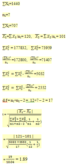
for t = 1.89 at 17 degree of freedom p > 0.05. Hence, the observed difference, gain in body weight due to two different types of diets is not significant. (Kulkarni S.K, 1999)
2.4 Typesof student t-test
There are two type ofstudent t-test-
(i) One -tailed test
(ii) Two-tailed test
The two-tailed test is generallyrecommended, because differencein either direction are usually importantto document. For example, it is obviously important to know ifa new treatment is significantly betterthan a standard or placebo treatment, butit is also important to know if a new treatment issignificantly worse and shouldtherefore be avoided.In this situation, the two-tailedtest provides an accepted criterion forwhen a difference shows thenew treatment to be either better or worse.
Sometimes, only a one-tailed test is needed. For example, that a new therapy is known to cost muchmore than the currently used therapy. Obviously, it would not be used if it were than the current therapy. Under these conditions, it acceptable to use a one- tailed test. When this occurs, the 5%rejection region for the null hypothesis is all put on one tail distribution, instead of being evenly divided between the extreme of the two tails.
In the one tailed test, the null hypothesis non rejection regionextends only to 1.645 standard errors above the ‘no difference’ point of 0. In the twotailed test, it extends to 1.96 standard errorsabove and below the ‘no difference’ point. This makes the one tailed test more robust-more able to detect a significant difference, if it is in the expected direction. (Jakel James et.al. 2001, Kothari C.R.1990)
2.5 Paired t-test
In many medical studies, individuals are followed over time to see if there is a change in the value of some continuous variable. Typically, this occurs in a “before and after” experiment, such as one testing to see if there was a drop in average blood pressure following treatment or to see if there was a drop in weight following the use of a special diet. In this type of comparison, an individual patient serves as his or her own control. This appropriate statistical test for this kind of data is the paired t-test. The paired is more robust than student’s t-test because it considers the variation from only one group of people, whereas the student’s t-test considers variation from two groups. Any variation that is detected in the paired t-test is attributable to the intervention or to changes over time in the same person.
2.6 Calculation of the value of t–
to calculate a paired t-test, a new variable is crated. This variable, called d, is the difference between the value before and after the intervention for each individual studied. The paired t-test is a test of the null hypothesis that, on the average, the difference is equal to 0, which is what be expected if there were no change over time. Using the symbol d? to indicate the mean observed difference between the before and after values, the formula for the paired t-test is as follows:
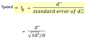
Degree of freedom df = N-1
The formula for the student’s t-test and the paired t-test are similer. The ratio of a difference to the variation around that difference (the standard error). In the student’s t-test, each of the two distribution to be compared contributers to the variation of the difference, and the two variance must be added. But in the paired t-test, there is only one frequency distribution, that of the before and after difference in each person. In the paired t-test, because only one mean is calculated (d?), only 1 degree of freedom is lost, therefore the formula for degree of freedom is N-1.
2.7 Interpretation of the results-
the value of t and their relationship to p are shown in a statistical table in the appendix. If the value of t is large, the p value will be small, because it is unlikely that is large t ratio will be obtained by chance alone. If the p value is 0.05 or less, it it is customary to assume that there is a real difference.(Jakel James et.al. 2001, Lachman Leon et.al. 1990)
References
1. Armstrong N. Anthony, James Kenneth C, “Pharmaceutical Experimental Design and Interpretation” 2006, Published by Taylor & Francis Ltd, London, Page no.14-16
2. Bolten Sanford, “pharmaceutical Stastics” Practical and clinical applications, Third edition, 2004, Published by Marcel Dekker Inc., New York, Page no 265 267,273
3. Jekel James F, et al., “Epidemiology, Biostatistics, and Preventive Medicine” Second edition 2001, Published by Saunders Publishers, Pennsylvania, Page no.160-163
4. Kothari C.R, “Research Methodology Method & Techniques” Second edition 1990, Published by New Age International Publishers, New Delhi, Page no.184, 195-196, 256-259
5. Kulkarni S.k, “Handbook of Experimental Pharmacology”, Third edition 1999, Published by Vallabh Prakashan, Delhi, Page no.175 -17
6. Lachman Leon, Lieberman Herbert, Kanig Joseph L, “The Theory and Practice of Industrial Pharmacy” Third edition 1990, Published by Varghese Publishing house, Dadar Bombey, Page no.269
7. Le Chap T, “Fundamental of Biostatistical Inference” Volume 124, 1992, Published by Marcel Dekker Inc, New York, Page no. 220-222
8. Student’s t-test procedure, biology.ed.ac.uk/research/groups/jdeacon/statistics/tress4a.html [accessed on 10 Aug.2012]
NOW YOU CAN ALSO PUBLISH YOUR ARTICLE ONLINE.
SUBMIT YOUR ARTICLE/PROJECT AT articles@pharmatutor.org
Subscribe to Pharmatutor Alerts by Email
FIND OUT MORE ARTICLES AT OUR DATABASE