EXPERIMENTAL DESIGN

ABOUT AUTHORS:
*Rakesh Gupta, Hemant Kumar Sharma, Manvendra Jaiswal, Rajeev Sharma, Narendra Nyola, Dr. Rajesh Yadav
Alwar Pharmacy College, M.I.A. Alwar,
Rajasthan, India 301001
rakeshapcpharma@gmail.com

ABSTRACT:
Experimental design is a planned interference in the natural order of events by the researcher. A selected condition or a change (treatment) is introduced. Observations or measurements are planned to illuminate the effect of any change in conditions. Complex designs, usually involving a number of "control groups," offer more information than a simple group design. It involves the Experimental Design and Data Analysis. The various type of experimental design, e.g. Statistical(Randomized Blocks, Latin Square, Factorial Design), Quasi Experimental (Time Series, Multiple Time Series), True Experimental (Pretest-Posttest Control Group, Post-test: Only Control Group, Solomon Four-Group), Pre-experimental (Static Group, One Group Pretest-Posttest, Experimental One-Shot Case Study).Process Models for DOE is common to begin with a process model of the `black box' type (Quadratic model & Linear model). Full factorial designs in two levels, Full factorial designs not recommended for 5 or more factors. Replication provides information on variability, Factor settings in standard order with replication, No randomization and no center points; Randomization provides protection against extraneous factors affecting the results. Contour plot Display 3-d surface on 2-d plot Vertical axis, Horizontal axis, Lines CCD designs start with a factorial or fractional factorial design (with centre points) and add "star" points to estimate curvature; A CCD design with k factors has 2k star points, 3 types of CCD designs, which depend on where the star points are placed Circumscribed (CCC), Inscribed (CCI), Face Cantered (CCF); the value of α is chosen to maintain rotatability.

REFERENCE ID: PHARMATUTOR-ART-2033

What is Experimental Design:-
Experimental design is a planned interference in the natural order of events by the researcher. He does something more than carefully observe what is occurring. This emphasis on experiment reflects the higher regard generally given to information so derived. There is good rationale for this. Much of the substantial gain in knowledge in all sciences has come from actively manipulating or interfering with the stream of events. There is more than just observation or measurement of a natural event. A selected condition or a change (treatment) is introduced. Observations or measurements are planned to illuminate the effect of any change in conditions.

The importance of experimental design also stems from the quest for inference about causes or relationships as opposed to simply description. Researchers are rarely satisfied to simply describe the events they observe. They want to make inferences about what produced, contributed to, or caused events. To gain such information without ambiguity, some form of experimental design is ordinarily required. As a consequence, the need for using rather elaborate designs ensues from the possibility of alternative relationships, consequences or causes. The purpose of the design is to rule out these alternative causes, leaving only the actual factor that is the real cause.

For example, Treatment A may have caused observed Consequences O, but possibly the consequence may have derived from Event E instead of the treatment or from Event E combined with the treatment. It is this pursuit of clear and unambiguous relationships that leads to the need for carefully planned designs.

The kinds of planned manipulation and observation called experimental design often seem to become a bit complicated. This is unfortunate but necessary, if we wish to pursue the potentially available information so the relationships investigated are clear and unambiguous. ^[1]

Considerations in Design Selection:-
The selection of a specific type of design depends primarily on both the nature and the extent of the information we want to obtain. Complex designs, usually involving a number of "control groups," offer more information than a simple group design. If "more information per project" were the sole criterion for selection of a design, we would be led to more and more complex designs. However, not all of the relevant information may be needed can be derived from any given design. Part of the information will be piggy-backed into the study by assumptions, some of which are explicit. Other information derives from a network of knowledge surrounding the project in question. Theories, accepted concepts, hypotheses, principles and empirical evidence from related studies contribute. To the extent that this knowledge is already available, the task of extracting the exact information needed to solve any research problem is circumscribed.

Collecting information is costly. The money and staff resources available have some limits. Subjects are usually found in finite quantities only. Time is a major constraint. The information to be gained has to be weighed against some estimate of the cost of collection. These points of two ways of checking potential designs:

1. What questions will this design answer? To do this, we must also be able to specify many of the questions the design won't answer as well ones it will answer. This should lead to a more realistic approach to experimental design than is usually given. Some simple and useful designs have been labelled as "poor" because they are relatively simple and will not answer some questions. Yet, they may provide clear and economical answers to the major questions of interest. Complex designs are not as useful for some purposes.

2. What is the relative information gain/cost picture? There is no specific formula or strategy for deriving some cut-off point in this regard. The major point here is that the researcher must take a close look at the probable cost before selecting a design. ^[2]

Experimental Design and Data Analysis:
The greatest challenge of toxicogenomics is no longer data generation but effective collection, management, analysis, and interpretation of data. Although genome sequencing projects have managed large quantities of data, genome sequencing deals with producing a reference sequence that is relatively static in the sense that it is largely independent of the tissue type analyzed or a particular stimulation. In contrast, transcriptomes, proteomes, and metabolisms are dynamic and their analysis must be linked to the state of the biologic samples under analysis. Further, genetic variation influences the response of an organism to a stimulus. Although the various toxicogenomic technologies (genomics, transcriptomics, proteomics, and metabolomics) survey different aspects of cellular responses, the approaches to experimental design and high-level data analysis are universal.

This chapter describes the essential elements of experimental design and data analysis for toxicogenomic experiments (Figure 1) and reviews issues associated with experimental design and data analysis. The discussion focuses on transcriptomics profiling using DNA microarrays. However, the approaches and issues discussed here apply to various toxicogenomic technologies and their applications. This chapter also describes the term biomarker.

EXPERIMENTAL DESIGN:
The types of biologic inferences that can be drawn from toxicogenomic experiments are fundamentally dependent on experimental design. The design must reflect the question that is being asked, the limitations of the experimental system, and the methods that will be used to analyze the data. Many experiments using global profiling approaches have been compromised by inadequate consideration of experimental design issues. ^[3]

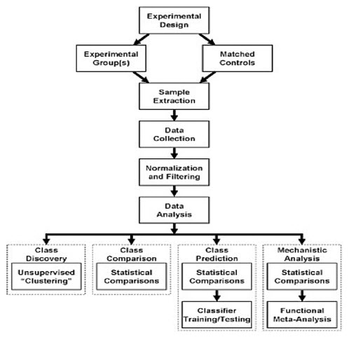
Figure:-1 Overview of the workflow in a toxicogenomic experiment. Regardless of the goal of the analysis, all share some common elements. However, the underlying experimental hypothesis, reflected in the ultimate goal of the analysis, should dictate the details of every step in the process, starting from the experimental design and extending beyond what is presented here to the methods used for validation.

TYPES OF EXPERIMENTS:-
DNA microarray experiments can be categorized into four types: class discovery, class comparison, class prediction, and mechanistic studies. Each type addresses a different goal and uses a different experimental design and analysis. Table summarizes the broad classes of experiments and representative examples of the data analysis tools that are useful for such analyses.

Table 1: - A Classification of Experimental Designs

1.Pre-experimental	2.True Experimental	3.Quasi Experimental	4.Statistical
Experimental One-Shot Case Study	Pre test-Post test Control Group	Time Series	Randomized Blocks
One Group Pre test-Post test	Post test: Only Control Group	Multiple Time Series	Latin Square
Static Group	Solomon Four-Group		Factorial Design

* One-Shot Case Study  X O₁

· A single group of test units is exposed to a treatment X

· A single measurement on the dependent variable is taken o₁

· There is no random assignment of test units

· The one-shot case study is more appropriate for exploratory than for conclusive research

* One Group Pre test-Post test O₁ X O₂

· A group of test units is measured twice

· There is no control group

· The treatment effect is computed as O₂ – O₁

· The validity of this conclusion is questionable since extraneous (unrelated)variables are largely uncontrolled

§  Static Group Design

EG:        X     O₁

CG:                O₂

· A two-group experimental design used, but only one of them is given the experimental treatment

· The experimental group (EG)is exposed to the treatment, and the control group (CG)is not

· Measurements on both groups are made only after the treatment

· Test units are not assigned at random

· The treatment effect would be measured as  O₁ – O₂

*  Pre test post test control group

  EG:           RO₁              O₂

   CG:           RO₃                      O₄

· Test units are randomly assigned to either the experimental or the control group

· A pre treatment measure is taken on each group

· The treatment effect is measured as: (o₂ - o₁) – (o₄-o₃)selection bias randomization

· The other extraneous effect is control as follows:

O₂ – O₁ =TE+H+MA+MT+I+SR+MO

O₄ – O₃ = H+MA+MT+I+SR+MO   =EV

· The experimental result is obtained by

(o₂ – o₁) – (o₄ – o₃) = TE + IT

· It is not controlled

* Post test only control group

EG:       R       X      O₁

CG:       R                O₂

TE = O₁ – O₂

· TE is obtained by of premeassurement implementation of design of pre-post-test design.

* Solomon four groups

                        R    O X O

                        R     O    O

                        R         X O

                        R             O

* Time series

O₁  O₂  O₃  O₄  O₅  X  O₆  O₇  O₈  O₉  O₁₀

· There is no randomization for test unit to treatment the timing of treatment presentation as well as which test unit are express may not be within the researcher central.

* Multiple Time Series

EG:        O₁  O₂  O₃  O₄  O₅     O₆  O₇  O₈  O₉  O₁₀

CG:       O₁  O₂  O₃  O₄  O₅  X  O₆  O₇  O₈  O₉  O₁₀

· If the controlled group carefully selected this design can be improvement over the simple time series experimental

· Can test the treatment effect tow ice again the pre-treatment measurement and again the controlled group

* Statistical Design

· Consist of a series of basic experiments that allow for statistical control and analysis of external variables and offer the following advantage:

- The effects of more than one independent variable can be measured

- Specific extraneous variables can be statistically controlled

- Economical designs can be formulated when each test unit is measured more than once

· The most common statistical designs are the randomized block design, the Latin square design, and the factorial design.

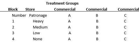
* Randomized Blocks

·  It is useful when there is only one major external variable, that might influence the dependent variable

· The test units are blocked, or grouped, on the basis of the external variable. 

· By blocking, the researcher ensures that the various experimental and control groups are matched closely on the external variable.^[4]

Treatment Groups

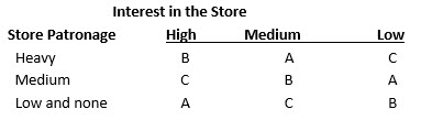
* Latin Square Design

• Allows the researcher to statistically control two non interacting external variablesas well as to manipulate the independent variable.
• Each external or blocking variable is divided into an equal number of blocks, or levels.
• The independent variable is also divided into the same number of levels.
• A Latin square is conceptualized as a table, with the rows and columns representing the blocks in the two external variables.
• The levels of the independent variable are assigned to the cells in the table.
• The assignment rule is that each level of the independent variable should appear only once in each row and each column.

Latin Square Design:-

Factorial Design
We may wish to try two kinds of treatments varied in two ways (called a 2x2 factorial design). Some factorial designs include both assignment of subjects (blocking) and several types of experimental treatment in the same experiment. When this is done it is considered to be a factorial design. A diagram of a 2x2 factorial design would look like:

R--GP--T-------O

      A1 B1

R--GP--T-------O

      A1 B2

R--GP--T-------O

      A2 B1

R--GP--T-------O

      A2 B2

The factorial design as we are describing is really a complete factorial design, rather than an incomplete factorial, of which there are several variations. The factorial is used when we wish information concerning the effects of different kinds or intensities of treatments. The factorial provides relatively economical information not only about the effects of each treatment, level or kind, but also about interaction effects of the treatment. In a single 2x2 factorial design similar to the one diagrammed above, information can be gained about the effects of each of the two treatments and the effect of the two levels within each treatment, and the interaction of the treatments. If all these are questions of interest, the factorial design is much more economical than running separate experiments.^[6]

It is used to measure the effects of two or more independent variables at various levels.

A factorial design may also be conceptualized as a table.

In a two-factor design, each level of one variable represents a row and each level of another variable represents a column.

Limitations of Experimentation:

• Experiments can be time consuming, particularly if the researcher is interested in measuring the long-term effects.
• Experiments are often expensive. The requirements of experimental group, control group, and multiple measurements significantly add to the cost of research.
• Experiments can be difficult to administer. It may be impossible to control for the effects of the extraneous variables, particularly in a field environment.
• Competitors may deliberately contaminate the results of a field experiment.

Process Models for DOE:-
Black box process model:- It is common to begin with a process model of the `black box' type, with several discrete or continuous input factors that can be controlled--that is, varied at will by the experimenter--and one or more measured output responses. The output responses are assumed continuous. Experimental data are used to derive an empirical (approximation) model linking the outputs and inputs. These empirical models generally contain first and second-order terms. Often the experiment has to account for a number of uncontrolled factors that may be discrete, such as different machines or operators, and/or continuous such as ambient temperature or humidity, Figure 2 illustrates this situation.

Schematic for a typical process with controlled inputs, outputs, discrete uncontrolled factors and continuous uncontrolled factors.

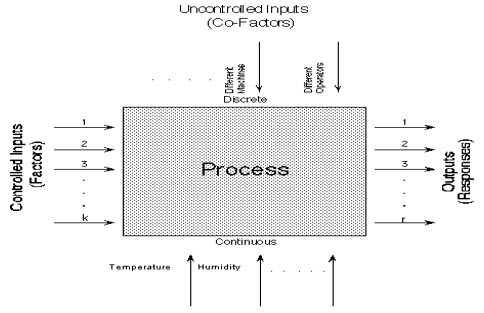
Figure 2:-A `Black Box' Process Model Schematic

Models for DOE's- The most common empirical models fit to the experimental data take either a linear form or quadratic form.

Linear model- A linear model with two factors, X₁ and X₂, can be written as:

Here, Y is the response for given levels of the main effects X₁ and X₂ and the X₁X₂ term is included to account for a possible interaction effect between X₁ and X₂. The constant ₀is the response of Y when both main effects are 0.

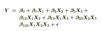
For a more complicated example, a linear model with three factors X₁, X₂, X₃ and one response, Y, would look like (if all possible terms were included in the model)-

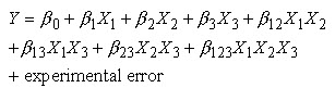
The three terms with single "X's" are the main effects terms. There are k(k-1)/2 = 3*2/2 = 3 two-way interaction terms and 1 three-way interaction term (which is often omitted, for simplicity). When the experimental data are analyzed, the entire unknown "" parameters are estimated and the coefficients of the "X" terms are tested to see which ones are significantly different from 0.

Quadratic model- A second-order (quadratic) model (typically used in response surface DOE's with suspected curvature) does not include the three-way interaction term but adds three more terms to the linear model, namely

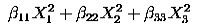
Note: Clearly, a full model could include many cross-product (or interaction) terms involving squared X's. However, in general these terms are not needed and most DOE software defaults to leaving them out of the model.

* Applications of DOE:
Choosing b/w alternatives (comparative experiment)
Selecting the key factors affecting a response (screening experiment)

Response surface modeling a process
-Hitting a target
-Maximizing or minimizing a response
-Making variation
-Seeking multiple goals

Regression modeling

Full factorial designs:
Full factorial designs in two levels-A design in which every setting of every factor appears with every setting of every other factor is a full factorial design.

A common experimental design is one with all input factors set at two levels each. These levels are called `high' and `low' or `+1' and `-1', respectively. A design with all possible high/low combinations of all the input factors is called a full factorial design in two levels. Ex- If there are k factors, each at 2 levels, a full factorial design has 2^k runs.

Table:-1  Number of Runs for a 2k Full Factorial
Number of Factors	Number of Runs
2	4
3	8
4	16
5	32
6	64
7	128

Full factorial designs not recommended for 5 or more factors- As shown by the above table, when the number of factors is 5 or greater, a full factorial design requires a large number of runs and are not very efficient. As recommended in the Design Guideline Table, a fractional factorial design or a Plackett-Burman design is a better choice for 5 or more factors.

* Two-Level Factorial Design: -
The simplest factorial design involves two factors, each at two levels. The top part of Figure 3 shows the layout of this two-by-two design, which forms the square “X-space” on the left. The equivalent one-factor-at-a-time (OFAT) experiment is shown at the upper right.

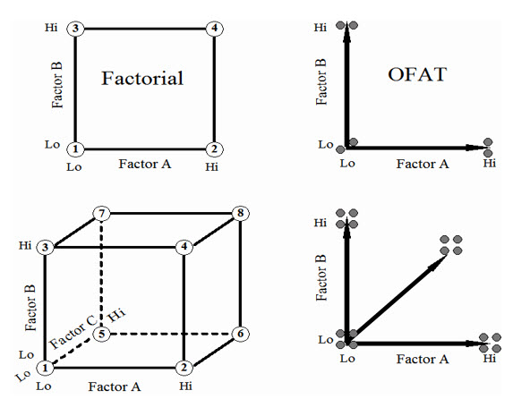
Figure 3 Two-Level Factorial Designs

A 2³ two-level, full factorial design; factors A B C

Table 2:- Full factorial design

Standard	Run	A	B	C
1	8	–	–	–
2	1	+	–	–
3	2	–	+	–
4	4	+	+	–
5	3	–	–	+
6	5	+	–	+
7	7	–	+	+
8	6	+	+	+

* Full Factorial Example:-
A full factorial design example:- An example of a full factorial design with 3 factors. The following is an example of a full factorial design with 3 factors that also illustrates replication, randomization, and added centre points. Suppose that we wish to improve the yield of a polishing operation. The three inputs (factors) that are considered important to the operation are Speed (X1), Feed (X2), and Depth (X3). We want to ascertain the relative importance of each of these factors on Yield (Y). Speed, Feed and Depth can all be varied continuously along their respective scales, from a low to a high setting. Yield is observed to vary smoothly when progressive changes are made to the inputs. This leads us to believe that the ultimate response surface for Y will be smooth.

Table 3:- High (+1), Low (-1), and Standard (0) Settings for a Polishing Operation

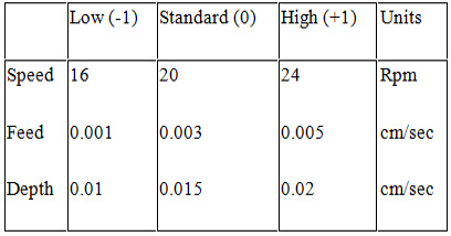
Factor Combinations: -Graphical representation of the factor level settings.

We want to try various combinations of these settings so as to establish the best way to run the polisher. There are eight different ways of combining high and low settings of Speed, Feed, and Depth. These eight are shown at the corners of the following diagram.

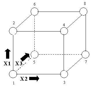
Figure 4:-A 2³ Two-level, Full Factorial Design; Factors X1, X2, X3. (The arrows show the direction of increase of the factors).

2³ implies 8 runs: -Note that if we have k factors, each run at two levels, there will be 2^k different combinations of the levels. In the present case, k= 3 and 2³ = 8.

Full Model: -Running the full complement of all possible factor combinations means that we can estimate all the main and interaction effects. There are three main effects, three two-factor interactions, and a three-factor interaction, all of which appear in the full model as follow:

A full factorial design allows us to estimate all eight `beta' coefficients.

Standard order: -The numbering of the corners of the box in the last figure refers to a standard way of writing down the settings of an experiment called `standard order'. We see standard order displayed in the following tabular representation of the eight-cornered box. Note that the factor settings have been coded, replacing the low setting by -1 and the high setting by 1.

Table 4:- A 2³ Two-level, Full Factorial Design Table Showing Runs in `Standard Order'

S.NO.	X1	X2	X3
1	-1	-1	-1
2	+1	-1	-1
3	-1	+1	-1
4	+1	+1	-1
5	-1	-1	+1
6	+1	-1	+1
7	-1	+1	+1
8	+1	+1	+1

Replication: Running the entire design more than once makes for easier data analysis because, for each run (i.e., `corner of the design box') we obtain an average value of the response as well as some idea about the dispersion (variability, consistency) of the response at that setting.

One of the usual analysis assumptions is that the response dispersion is uniform across the experimental space. The technical term is `homogeneity of variance'. Replication allows us to check this assumption and possibly find the setting combinations that give inconsistent yields, allowing us to avoid that area of the factor space.

We now have constructed a design table for a two-level full factorial in three factors, replicated twice.

Table 5:-The 2³ Full Factorial Replicated Twice and Presented in Standard Order.

Table 5:-The 23 Full Factorial Replicated Twice and Presented in Standard Order.

S. no.	Speed, X1	Feed, X2	Depth, X3
1	16, -1	.001, -1	.01, -1
2	24, +1	.001, -1	.01, -1
3	16, -1	.005, +1	.01, -1
4	24, +1	.005, +1	.01, -1
5	16, -1	.001, -1	.02, +1
6	24, +1	.001, -1	.02, +1
7	16, -1	.005, +1	.02, +1
8	24, +1	.005, +1	.02, +1
9	16, -1	.001, -1	.01, -1
10	24, +1	.001, -1	.01, -1
11	16, -1	.005, +1	.01, -1
12	24, +1	.005, +1	.01, -1
13	16, -1	.001, -1	.02, +1
14	24, +1	.001, -1	.02, +1
15	16, -1	.005, +1	.02, +1
16	24, +1	.005, +1	.02, +1

Randomization:- If we now ran the design as is, in the order shown, we would have two deficiencies, namely: No randomization, and No center points.

The more freely one can randomize experimental runs, the more insurance one has against extraneous factors possibly affecting the results, and hence perhaps wasting our experimental time and effort. For example, consider the `Depth' column: the settings of Depth, in standard order, follow a `four low, four high, four low, four high' pattern. Suppose now that four settings are run in the day and four at night, and that (unknown to the experimenter) ambient temperature in the polishing shop affects Yield. We would run the experiment over two days and two nights and conclude that Depth influenced Yield, when in fact ambient temperature was the significant influence. So the moral is: Randomize experimental runs as much as possible.

Randomization provides protection against extraneous factors affecting the results.

Table 6:-The 23 Full Factorial Replicated Twice with Random Run Order Indicated.

Random Order	Standard Order	X1	X2	X3
1	5	-1	-1	+1
2	15	-1	+1	+1
3	9	-1	-1	-1
4	7	-1	+1	+1
5	3	-1	+1	-1
6	12	+1	+1	-1
7	6	+1	-1	+1
8	4	+1	+1	-1
9	2	+1	-1	-1
10	13	-1	-1	+1
11	8	+1	+1	+1
12	16	+1	+1	+1
13	1	-1	-1	-1
14	14	+1	-1	+1
15	11	-1	+1	-1
16	10	+1	-1	-1

Table showing design matrix with randomization and centre points.This design would be improved by adding at least 3 centre point runs placed at the beginning, middle and end of the experiment. The final design matrix is shown below Table 7.

Table 7:- The 23 Full Factorial Replicated Twice with Random Run Order Indicated and Centre Point Runs Added

Random Order	Standard Order	X1	X2	X3
1		0	0	0
2	5	-1	-1	+1
3	15	-1	+1	+1
4	9	-1	-1	-1
5	7	-1	+1	+1
6	3	-1	+1	-1
7	12	+1	+1	-1
8	6	+1	-1	+1
9		0	0	0
10	4	+1	+1	-1
11	2	+1	-1	-1
12	13	-1	-1	+1
13	8	+1	+1	+1
14	16	+1	+1	+1
15	1	-1	-1	-1
16	14	+1	-1	+1
17	11	-1	+1	-1
18	10	+1	-1	-1
19		0	0	0

 

5. Contour Plot:- A contour plot is a graphical technique for representing a 3-dimensional surface by plotting constant z slices, called contours, on a 2-dimensional format. That is, given a value for z, lines are drawn for connecting the (x, y) coordinates where that z value occurs.

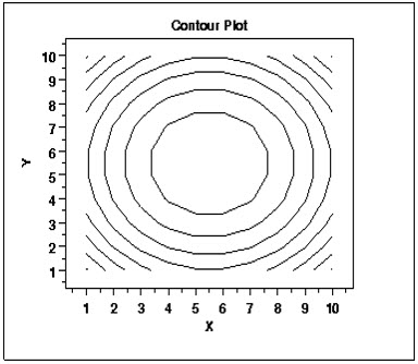
Figure 5:- The contour plot is an alternative to a 3-D surface plot.

• Definition:- This contour plot shows that the surface is symmetric and peaks in the centre. The contour plot is formed by:-

Vertical axis: Independent variable 2

Horizontal axis: Independent variable 1

Lines: iso-response values

The independent variables are usually restricted to a regular grid. The actual techniques for determining the correct iso-response values are rather complex and are almost always computer generated. An additional variable may be required to specify the Z values for drawing the iso-lines. Some software packages require explicit values. Other software packages will determine them automatically.

If the data (or function) do not form a regular grid, you typically need to perform a 2-D interpolation to form a regular grid.

• Questions:- The contour plot is used to answer the question. How does Z change as a function of X and Y?
• Importance:- Visualizing 3-dimensional data, For univariate data, a run sequence plot and a histogram are considered necessary first steps in understanding the data. For 2-dimensional data, a scatter plot is a necessary first step in understanding the data.

In a similar manner, 3-dimensional data should be plotted. Small data sets, such as result from designed experiments, can typically be represented by block plots, dex mean plots, and the like (here, "DEX" stands for "Design of Experiments"). For large data sets, a contour plot or a 3-D surface plot should be considered a necessary first step in understanding the data.

• DEX Contour Plot:- The dex contour plot is a specialized contour plot used in the design of experiments. In particular, it is useful for full and fractional designs.
• Software:- Contour plots are available in most general purpose statistical software programs. They are also available in many general purpose graphics and mathematics programs. These programs vary widely in the capabilities for the contour plots they generate. Many provide just a basic contour plot over a rectangular grid while others permit color filled or shaded contours. Dataplotsupports a fairly basic contour plot. Most statistical software programs that support design of experiments will provide a dex contour plot capability.

5. Central Composite Designs (CCD):-

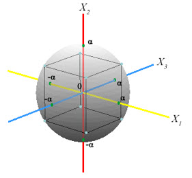
Figure 6:- CCD

Box-Wilson Central Composite Designs:-

CCD designs start with a factorial or fractional factorial design (with centre points) and add "star" points to estimate curvature.

 A Box-Wilson Central Composite Design, commonly called `a central composite design,' contains an imbedded factorial or fractional factorial design with centre points that is augmented with a group of `star points' that allow estimation of curvature. If the distance from the canter of the design space to a factorial point is ±1 unit for each factor, the distance from the centre of the design space to a star point is ±α with |α| > 1. The precise value of α depends on certain properties desired for the design and on the number of factors involved.

Similarly, the number of centre point runs the design is to contain also depends on certain properties required for the design.

Diagram of central composite design generation for two factors-

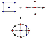
Figure 7:- Generation of a Central Composite Design for Two Factors

A CCD design with k factors has 2k star points. A central composite design always contains twice as many star points as there are factors in the design. The star points represent new extreme values (low and high) for each factor in the design. Table 7 summarizes the properties of the three varieties of central composite designs. Figure 7 illustrates the relationships among these varieties.

Description of 3 types of CCD designs, which depend on where the star points are placed.

Table 8:- Central Composite Designs
Central Composite  Design Type	Terminology	Comments
Circumscribed	CCC	CCC designs are the original form of the central composite design. The star points are α at some distance α from the centre based on the properties desired for the design and the number of factors in the design. The star points establish new extremes for the low and high settings for all factors. Figure 5 illustrates a CCC design. These designs have circular, spherical, or hyper spherical symmetry and require 5 levels for each factor. Augmenting an existing factorial or resolution V fractional factorial design with star points can produce this design.
Inscribed	CCI	For those situations in which the limits specified for factor settings are truly limits, the CCI design uses the factor settings as the star points and creates a factorial or fractional factorial design within those limits (in other words, a CCI design is a scaled down CCC design with each factor level of the CCC design divided by α to generate the CCI design). This design also requires 5 levels of each factor.
Face Centered	CCF	In this design the star points are at the center of each face of the factorial space, so α = ± 1. This variety requires 3 levels of each factor. Augmenting an existing factorial or resolution V design with appropriate star points can also produce this design.

 

Pictorial representation of where the star points are placed for the 3 types of CCD designs-

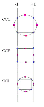
Figure 8:- Comparison of the Three Types of Central Composite Designs.

Comparison of the 3 central composite designs. The diagrams in Figure 8 illustrate the three types of central composite designs for two factors. Note that the CCC explores the largest process space and the CCI explores the smallest process space. Both the CCC and CCI are rotatable designs, but the CCF is not. In the CCC design, the design points describe a circle circumscribed about the factorial square. For three factors, the CCC design points describe a sphere around the factorial cube.[6]

Determining α in Central Composite Designs-

The value of α is chosen to maintain rotatability. To maintain rotatability, the value of α depends on the number of experimental runs in the factorial portion of the central composite design:

α = [number of factorial runs]1/4

If the factorial is a full factorial, then

α = [2k]1/4

However, the factorial portion can also be a fractional factorial design of resolution V. Table 8 illustrates some typical values of α as a function of the number of factors.

Values of α depending on the number of factors in the factorial part of the design

Table 9:- Determining α for Rotatability
Number of Factors	Factorial Portion	Scaled Value for   Relative to ±1
2	22	22/4 = 1.414
3	23	23/4 = 1.682
4	24	24/4 = 2.000
5	25-1	24/4 = 2.000
5	25	25/4 = 2.378
6	26-1	25/4 = 2.378
6	26	26/4 = 2.828

Orthogonal blocking:- The value of α also depends on whether or not the design is orthogonally blocked. That is, the question is whether or not the design is divided into blocks such that the block effects do not affect the estimates of the coefficients in the 2nd order model.

Example of both rotatability and orthogonal blocking for two factors under some circumstances, the value of α allows simultaneous rotatability and orthogonality. One such example for k = 2 are shown below:

Table 10:- rotatability and orthogonal blocking for two factors

BLOCK	X1	X2
1	-1	-1
1	1	-1
1	-1	1
1	1	1
1	0	0
1	0	0
2	-1.414	0
2	1.414	0
2	0	-1.414
2	0	1.414
2	0	0
2	0	0

Additional central composite designs Examples of other central composite designs will be given after Box-Behnken designs are described.[6]

References:-
1. Brownlee, K. A. Statistical theory and methodology in science and engineering. New York: Wiley, 1960.
2. Campbell, D. and Stanley J. Experimental and quasi-experimental designs for research and teaching. In Gage (Ed.), Handbook on research on teaching. Chicago: Rand McNally & Co., 1963.
3.Simon, R., M.D. Radmacher, and K. Dobbin. 2002. Design of studies using DNA microarrays. Genet. Epidemiol. 23(1):21-36.
Churchill, G.A. 2002. Fundamentals of experimental design for cDNA microarrays. Nat. Genet. 32(Suppl.):490-495. © 4th ed. 2006 Dr. Rick Yount.
4. Box, G.E., Hunter,W.G., Hunter, J.S., Statistics for Experimenters: Design, Innovation, and Discovery, 2nd Edition, Wiley, 2005, ISBN 0-471-71813-0.
5. Watson, David F., Contouring: A Guide to the Analysis and Display of Spatial Data, 340 pp., Pergamon Press, New York, 1992.(ccd).